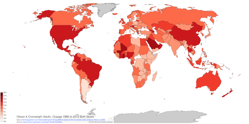
Obese and Overweight Adults¶

This notebook shows how to process data on obesity and overweight published by the Guardian to create Web based maps.

In [1]:

import io
import requests
import pandas as pd

from geonamescache.mappers import country
country_name_to_iso3 = country(from_key='name', to_key='iso3')

df = pd.read_excel('data/Overweight and Obesity data - IHME.xlsx', 'Obesity Overweight Adults', skiprows=1)
df.head()

Out[1]:

	country	Prevalence 1980 Male ≥ 20	Prevalence 1980 Female ≥ 20	Prevalence 1980 Both Sexes ≥ 20	Rank 1980 Both Sexes ≥ 20	Prevalence 1990 Male ≥ 20	Prevalence 1990 Female ≥ 20	Prevalence 1990 Both Sexes ≥ 20	Prevalence 2000 Male ≥ 20	Prevalence 2000 Female ≥ 20	Prevalence 2000 Both Sexes ≥ 20	Rank 2000 Both Sexes ≥ 20	Prevalence 2013 Male ≥ 20	Prevalence 2013 Female ≥ 20	Prevalence 2013 Both Sexes ≥ 20	Rank 2013 Both Sexes ≥ 20	Change 1980 to 2013, Males ≥ 20	Change 1980 to 2013, Females ≥ 20	Change 1980 to 2013 Both Sexes ≥ 20
0	Global	0.288467	0.297723	0.293944	NaN	0.298300	0.307592	0.303699	0.334921	0.349454	0.342819	NaN	0.368668	0.380008	0.374837	NaN	0.080201	0.082285	0.080893
1	Afghanistan	0.434719	0.382357	0.408788	101	0.461357	0.403985	0.433378	0.479945	0.418287	0.449724	102	0.492275	0.426127	0.459428	113	0.057556	0.043770	0.050639
2	Angola	0.364258	0.414418	0.391533	109	0.336723	0.391192	0.366153	0.365469	0.425857	0.397884	123	0.428890	0.490836	0.461870	111	0.064633	0.076418	0.070337
3	Albania	0.465603	0.378795	0.424249	93	0.468094	0.379045	0.425124	0.503193	0.405219	0.453366	98	0.561735	0.458180	0.510192	96	0.096132	0.079384	0.085943
4	Andorra	0.402356	0.362815	0.382455	115	0.411833	0.373189	0.392384	0.355085	0.347157	0.351926	132	0.344056	0.361205	0.353715	139	-0.058301	-0.001610	-0.028740

5 rows × 19 columns

Create iso column from country names, then set country to index, so it can be easily omitted when saving.

In [2]:

df['iso3'] = df['country'].apply(country_name_to_iso3)
df.dropna(subset=['iso3'], inplace=True)
df.set_index('country', inplace=True)

Remove all Rank columns, as they are useless in the map display. Also remove repeating info from column names.

In [3]:

for col in df.columns:
    if col.startswith('Rank'):
        del df[col]

df.columns = df.columns.map(lambda x: x.replace('  ≥ 20', ''))

Convert float values back to percentages as integers.

In [4]:

def percentage(x):
    if isinstance(x, float) and not np.isnan(x):
        x = int(x * 100)
    return x

df.applymap(percentage)
df.sort('Prevalence 2013 Both Sexes', ascending=False).head(20)

Out[4]:

	Prevalence 1980 Male	Prevalence 1980 Female	Prevalence 1980 Both Sexes	Prevalence 1990 Male	Prevalence 1990 Female	Prevalence 1990 Both Sexes	Prevalence 2000 Male	Prevalence 2000 Female	Prevalence 2000 Both Sexes	Prevalence 2013 Male	Prevalence 2013 Female	Prevalence 2013 Both Sexes	Change 1980 to 2013, Males	Change 1980 to 2013, Females	Change 1980 to 2013 Both Sexes	iso3
country
Tonga	0.772975	0.835758	0.804527	0.795270	0.853557	0.825235	0.817666	0.871935	0.846015	0.835377	0.883101	0.860597	0.062402	0.047344	0.056070	TON
Samoa	0.774268	0.798372	0.786354	0.787211	0.812553	0.799941	0.803319	0.830005	0.815938	0.830393	0.850131	0.839602	0.056125	0.051759	0.053249	WSM
Kiribati	0.735279	0.788322	0.761686	0.720434	0.781147	0.750673	0.738880	0.798411	0.768659	0.764518	0.818109	0.791152	0.029238	0.029788	0.029466	KIR
Kuwait	0.645810	0.772501	0.694059	0.618879	0.754681	0.675844	0.704987	0.812580	0.744450	0.744678	0.843116	0.780510	0.098868	0.070615	0.086451	KWT
Qatar	0.709360	0.742005	0.725359	0.749240	0.768749	0.757736	0.752717	0.779269	0.759686	0.756589	0.785497	0.770650	0.047229	0.043492	0.045291	QAT
Marshall Islands	0.592824	0.678309	0.635918	0.624106	0.706842	0.666693	0.710314	0.793677	0.753373	0.727467	0.807505	0.768888	0.134643	0.129196	0.132970	MHL
Egypt	0.631427	0.638216	0.635433	0.691683	0.675286	0.684057	0.707959	0.770306	0.739015	0.711999	0.794318	0.752854	0.080572	0.156102	0.117421	EGY
Federated States of Micronesia	0.594243	0.778843	0.686701	0.604084	0.788749	0.696181	0.612832	0.807107	0.712016	0.656903	0.841558	0.748792	0.062660	0.062715	0.062091	FSM
Libya	0.685628	0.755857	0.718560	0.694088	0.760965	0.725364	0.696418	0.762567	0.728262	0.706405	0.770430	0.739099	0.020777	0.014573	0.020539	LBY
Jordan	0.645657	0.670758	0.658486	0.682612	0.702582	0.693227	0.696453	0.726638	0.711315	0.716322	0.756393	0.736276	0.070664	0.085635	0.077790	JOR
Palestine	0.560601	0.669348	0.616366	0.606482	0.703151	0.655955	0.647779	0.734397	0.692048	0.699748	0.770494	0.735780	0.139146	0.101145	0.119414	PSE
Syria	0.647304	0.667149	0.657267	0.662187	0.679184	0.670557	0.686338	0.698093	0.692298	0.719710	0.726530	0.723239	0.072407	0.059381	0.065972	SYR
Saudi Arabia	0.490339	0.573332	0.527182	0.546685	0.616445	0.573981	0.663885	0.713937	0.685833	0.690043	0.742164	0.711451	0.199704	0.168832	0.184269	SAU
Bahrain	0.352026	0.619103	0.461056	0.434211	0.668254	0.530606	0.608020	0.709692	0.653509	0.676819	0.751828	0.710868	0.324793	0.132725	0.249812	BHR
Mexico	0.517496	0.536316	0.528388	0.556735	0.561022	0.559975	0.616951	0.674427	0.647707	0.668073	0.714038	0.693023	0.150577	0.177723	0.164635	MEX
Paraguay	0.589067	0.695285	0.645313	0.593625	0.700287	0.649113	0.620579	0.720989	0.671923	0.628614	0.729518	0.679937	0.039546	0.034233	0.034624	PRY
Iceland	0.667173	0.520689	0.594408	0.671113	0.524359	0.598084	0.703088	0.563824	0.633428	0.736479	0.608653	0.671341	0.069307	0.087964	0.076933	ISL
Belize	0.551820	0.726283	0.638491	0.551675	0.725683	0.638214	0.565368	0.738342	0.652606	0.586480	0.752715	0.671269	0.034660	0.026432	0.032778	BLZ
Lebanon	0.586627	0.526342	0.555342	0.655865	0.589850	0.620963	0.683565	0.607520	0.644769	0.711430	0.623260	0.666878	0.124803	0.096919	0.111535	LBN
United States	0.567312	0.439402	0.501213	0.607483	0.491306	0.547930	0.676886	0.583662	0.629212	0.709383	0.618972	0.663268	0.142071	0.179570	0.162055	USA

20 rows × 16 columns

Save data as CSV, and output column list.

In [5]:

df.to_csv('../static/data/csv/obese-overweight-adults-countries.csv', encoding='utf-8', index=False)
', '.join(["'%s'" % col for col in df.columns if col != 'iso3'])

Out[5]:

"'Prevalence 1980 Male', 'Prevalence 1980 Female', 'Prevalence 1980 Both Sexes', 'Prevalence 1990 Male', 'Prevalence 1990 Female', 'Prevalence 1990 Both Sexes', 'Prevalence 2000 Male', 'Prevalence 2000 Female', 'Prevalence 2000 Both Sexes', 'Prevalence 2013 Male', 'Prevalence 2013 Female', 'Prevalence 2013 Both Sexes', 'Change 1980 to 2013, Males', 'Change 1980 to 2013, Females', 'Change 1980 to 2013 Both Sexes'"

Obese and Overweight Adults¶

Volcano Map Poster

Recommended Books

Map Preview

Obese & Overweight Adults: Change 1980 to 2013 Both Sexes

About this post